PACTOT model¶

The PACTOT (Process ACTivity – Object Trade) model is based on linear constrained optimization. It was developed for the UK material flow mapping project, and then extracted here.

Model structure¶

One possible representation of processes is to define their “recipe”, that is the material inputs and outputs associated with the operation of the process.

(1)¶\[\begin{align} u_{ij} &= \text{use of material $i$ in process $j$} \\ s_{ij} &= \text{supply of material $i$ from process $j$} \end{align}\]

For example, the processes in this figure: 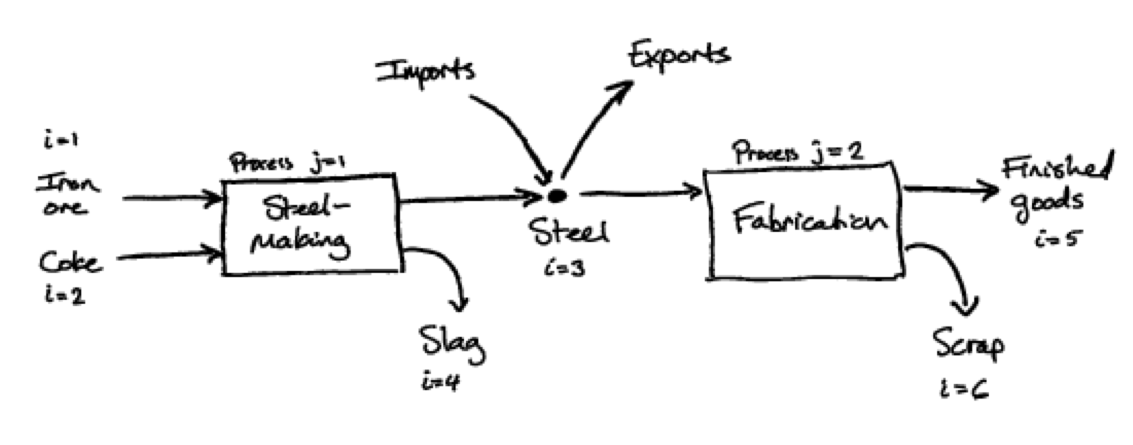System sketch can be defined as:

(2)¶\[\begin{align} U_1 &= \begin{bmatrix} 0.8 \\ 0.2 \\ 0 \\ 0 \\ 0 \\ 0 \end{bmatrix} & S_1 &= \begin{bmatrix} 0 \\ 0 \\ 0.9 \\ 0.1 \\ 0 \\ 0 \end{bmatrix} \\[0.5em] U_2 &= \begin{bmatrix} 0 \\ 0 \\ 1 \\ 0 \\ 0 \\ 0 \end{bmatrix} & S_2 &= \begin{bmatrix} 0 \\ 0 \\ 0 \\ 0 \\ 0.7 \\ 0.7 \end{bmatrix} \end{align}\]

which describes, for example, that 70% of the output of the “rolling” process is finished goods, while 30% is scrap.

If the scale of operation of each process is $X_j$, then the inputs and outputs of material $i$ are $u_{ij} X_j$ and $s_{ij} X_j$ respectively.

In addition, there may be imports $v_i$ and exports $w_i$ of some materials. In the example diagram, this applies only to material $i = 3$.

Finally, conservation of mass should apply for the intermediate materials (in this case $i = 3$):

\[ \sum_j s_{ij} X_j - \sum_j u_{ij} X_j + v_i - w_i = 0 \]

The problem is to determine the flows (i.e. the size of the arrows on the diagram), such that the conservation equation(s) are satisfied, while accounting for any [uncertain] data that may be available.

Constraint matrices¶

The model variables are listed in a vector $z$:

\[\begin{split} \boldsymbol{z} = \begin{bmatrix} \hat{\boldsymbol{x}} \\ \hat{\boldsymbol{v}} \\ \hat{\boldsymbol{w}} \\ \boldsymbol{\rho} \end{bmatrix} \end{split}\]

Because the magnitude of the flows of different objects may vary by orders of magnitude, the model is set up to use normalised variables. Each object type $i$ has a representative scale $K_i$. The scale of the process activity $K_j$ is defined relative to the scale of the process’s main input or output. So:

(3)¶\[\begin{align} x_j &= K_j \hat{x}_j \\ v_i &= K_i \hat{v}_i \\ w_i &= K_i \hat{w}_i \\ \rho_i &= K_i \hat{\rho}_i \end{align}\]

These constraints are encoded into constraint matrices of the form $\boldsymbol{C} \boldsymbol{z} = \boldsymbol{v}$.

First, objects must balance:

(4)¶\[\begin{align} \boldsymbol{C}_1 &= \begin{bmatrix} \boldsymbol{S} - \boldsymbol{U} & \boldsymbol{I} & -\boldsymbol{I} & \boldsymbol{0} \end{bmatrix} \\ \boldsymbol{v}_1 &= \boldsymbol{0} \end{align}\]

where the 4 sub-matrices correspond to $\hat{\boldsymbol{x}}$, $\hat{\boldsymbol{v}}$, $\hat{\boldsymbol{w}}$, and $\boldsymbol{\rho}$ respectively.

Second, some processes are expected to balance:

(5)¶\[\begin{align} \boldsymbol{C}_2 &= \begin{bmatrix} \boldsymbol{0} & \boldsymbol{0} & \boldsymbol{0} & (\boldsymbol{S}_\text{bal} - \boldsymbol{U}_\text{bal})^{\mathrm{T}} \end{bmatrix} \\ \boldsymbol{v}_2 &= \boldsymbol{0} \end{align}\]

where the subscript “bal” indicates the subset of columns corresponding to processes which should be expected to balance.

Thirdly, the density should be 1 for objects which are measured in kg:

(6)¶\[\begin{align} \boldsymbol{C}_3 &= \begin{bmatrix} \boldsymbol{0} & \boldsymbol{0} & \boldsymbol{0} & \boldsymbol{I}_\text{kg} \end{bmatrix} \\ \boldsymbol{v}_3 &= \boldsymbol{I}_\text{kg} \end{align}\]

where, similarly, the subscript “kg” indicates the subset of rows corresponding to objects which are measured in kg.

Finally, the import and export flows should be zero for objects which are not traded:

(7)¶\[\begin{align} \boldsymbol{C}_4 &= \begin{bmatrix} \boldsymbol{0} & \boldsymbol{I}_\text{no trade} & \boldsymbol{0} & \boldsymbol{0} \\ \boldsymbol{0} & \boldsymbol{0} & \boldsymbol{I}_\text{no trade} & \boldsymbol{0} \\ \end{bmatrix} \\ \boldsymbol{v}_4 &= \boldsymbol{0} \end{align}\]

where, again, the subscript “no trade” indicates the subset of rows corresponding to objects which are not traded.

These constraint matrices are stacked to form the complete set of constraints:

(8)¶\[\begin{align} \boldsymbol{C} &= \begin{bmatrix} \boldsymbol{C}_1 \\ \boldsymbol{C}_2 \\ \boldsymbol{C}_3 \\ \boldsymbol{C}_4 \end{bmatrix} & \boldsymbol{v} &= \begin{bmatrix} \boldsymbol{v}_1 \\ \boldsymbol{v}_2 \\ \boldsymbol{v}_3 \\ \boldsymbol{v}_4 \end{bmatrix} \end{align}\]

Cost function¶

The variables are solved in a least-squares optimisation, minimising the weighted residual error in the observed data values:

\[ r_k(\boldsymbol{z}) = D_k - g_k(\boldsymbol{z}) \]

where $D_k$ is the measured value for observation $k$, and $g_k$ is the function describing what the observation is measuring.

The cost function is

\[ S(\boldsymbol{z}) = \sum_k W_k r_k(\boldsymbol{z})^2 \]

which should be minimised within the constraints described above.

The weight $W_k$ is currently simply the numerical “quality” score assigned to the observation.

Observation types¶

Different types of observation measure different aspects of the system.

Process input observation of object $i$ into process $j$: $g_k = u_{ij} x_{j} $
Process output observation of object $i$ from process $j$: $g_k = s_{ij} x_{j} $
Import observation of object $i$: $g_k = v_{i} $
Export observation of object $i$: $g_k = w_{i} $

It’s also convenient to describe some more complex observations, which match the data that is sometimes available:

Consumption observation of object $i$ is the sum of all inputs: $g_k = \sum_j u_{ij} x_{j}$
Production observation of object $i$ is the sum of all outputs: $g_k = \sum_j s_{ij} x_{j}$

In the code, the measurement function $g_k$ is represented by a matrix multiplication:

\[ g_k(\boldsymbol{z}) = \boldsymbol{d}_k^\mathrm{T} \boldsymbol{z} \]

Observation (\(k\))	Model variable \(g_k\)	Value \(D_k\)
Input of iron ore	\(u_{11} X_{1}\)	\(= 80\)
Input of coke	\(u_{21} X_{1}\)	\(= 30\)
Imports of steel	\(v_{3}\)	\(= 50\)
Exports of steel	\(w_{3}\)	\(< 20\)
Production of final goods	\(s_{62} X_{2}\)	\(= 90\)

probs-models

PACTOT model

Contents

PACTOT model¶

Model structure¶

Constraint matrices¶

Cost function¶

Observation types¶

Example¶